"Key Ingredients" of Deep Learning
Breaking down deep learning's 4 central components
By Evan Meade, 2020-01-07

Until very recently, I used the terms “deep learning,” “machine learning,” and “artificial intelligence” interchangeably to describe basically any algorithm which seemed to adjust itself automatically using data. Somewhere in that opaque process, I assumed there must be a kind of magical force guiding the code towards a more efficient form, since I had no real understanding of how such systems worked. Luckily, I recently read a book which helped introduce me to the revolutionary field of deep learning while remaining quite readable and accessible.
That book, of course, is the aptly titled Deep Learning, by John D. Kelleher, which belongs to the MIT Press Essential Knowledge series (cover above © 2019 The Massachusetts Institute of Technology). The goal of the short-ish book is to provide an accurate, yet non-technical introduction to the field of deep neural networks. In my opinion, it does a great job of explaining the field’s central concepts, though some chapters are admittedly more equation heavy than others. With this article, I hope to distill and clarify some of the book’s major insights both for those who were left with questions after reading it, and for those who are simply too busy to read it in the first place.
The first crucial part of this book is its explanation of the relationships and differences between the three terms I mentioned at the beginning: “deep learning,” “machine learning,” and “artificial intelligence.” Much to my surprise, they are actually not synonyms, though their definitions do overlap. Rather, they are subfields of one another, in a nested relationship as shown by this Venn diagram:
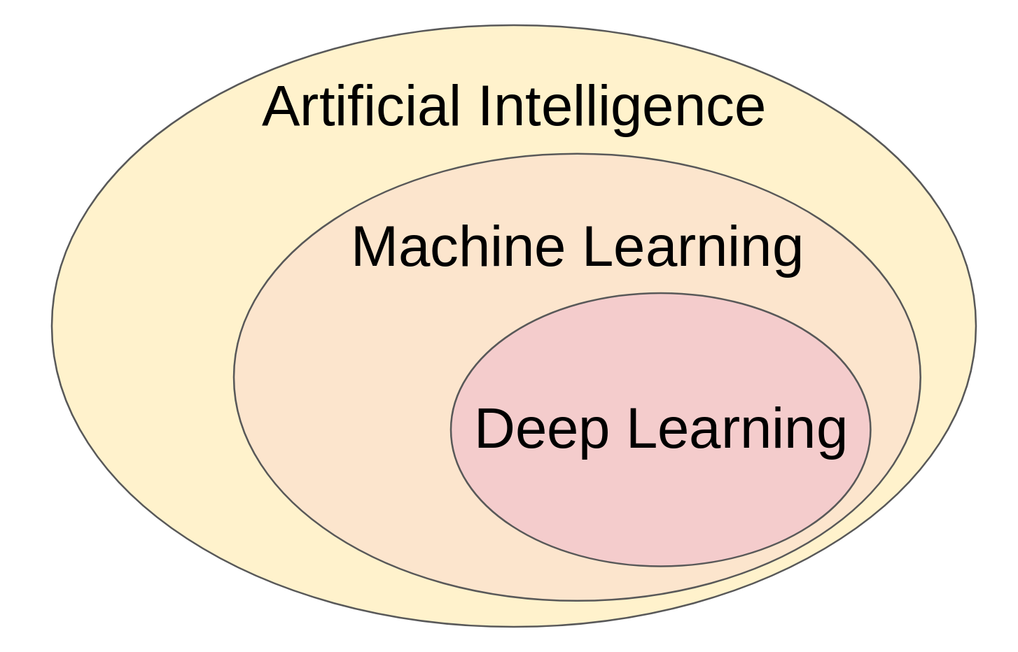
Deep learning Venn diagram; based on Figure 1.1 from Deep Learning (2019)
Thus, rather than being equivalent terms, each one describes a more specific kind of algorithm:
- Artificial Intelligence (AI) – Very broad term describing algorithms that enable machines to learn, reason, and problem solve in a manner understandable to humans
- Machine Learning – AI algorithms which “learn” from data by matching a given dataset with the best fitting function from a given set of functions
- Deep Learning – Machine learning algorithms based on neural networks which have 2 or more “hidden” layers (sometimes they have hundreds)
So essentially, artificial intelligence describes all projects which have the goal of getting machines to think and act like humans. Machine learning then refers to a specific approach and subfield of AI which trains machines to “learn” from patterns in datasets. The most specific term, deep learning, refers to machine learning conducted using a particular kind of model called a deep neural network to represent the machine’s “brain.”
Another key takeaway from early on is what these algorithms are actually used for. Machine learning tasks are generally broken down into one of three categories. The most common type is “supervised learning,” where the algorithm is trained to match a given set of inputs to a given set of outputs. For instance, training a program to differentiate pictures of dogs and cats using labeled images would be a form of supervised learning. However, one drawback of this kind of learning is that annotating large datasets with the desired outputs can be very expensive. Another option would be to use “unsupervised learning,” where the algorithm “clusters” similar sets of inputs together, without being given a desired output. To follow the prior analogy, this would involve the program finding groups of images with similar kinds of features. These may happen to line up with the desired output of cats and dogs, or they may provide new insights into the data altogether.
Finally, there is “reinforcement learning,” which is the strange middle ground between the other types of machine learning. This would describe learning where there is a desired end goal, but no specifically desired path to get there. The best example of this would be a program trained to play a complex board game, such as Go. In this game, 2 opponents take turns placing stones on a 19×19 grid, with the goal of surrounding more territory than the opponent. The goal is clear: surround more area than the opponent. However, this requires a large number of moves, each of which invites a large number of possibilities. In short, it is very difficult to judge a particular move as “correct,” though it is trivial to judge a game’s result as “correct.” Advanced methods are used in reinforcement learning to train programs in these kinds of scenarios.
In summary, there are 3 approaches to machine learning, each of which has a different use case:
- Supervised learning – matches inputs to a known output
- Unsupervised learning – clusters similar inputs together
- Reinforcement learning – achieves defined goals using undefined strategies to get there
I know, there are a lot of different parts to all this between the goal and the data and the functions and whatever a neural network is. It can be easy to feel lost in all these overlapping terms, and not know what really goes into the process of deep learning. In my opinion, a great roadmap to exploring all this comes near the beginning of this book, where Kelleher describes the central components of the field:
"The three key ingredients in machine learning [are]:
1. Data (a set of historical examples).
2. A set of functions that the algorithm will search through to find the best match with the data.
3. Some measure of fitness that can be used to evaluate how well each candidate function matches the data.
All three of these ingredients must be correct if a machine learning project is to succeed…”
At its most fundamental level, these really are the key ingredients of machine learning. To that I would only add one more ingredient:
"4. A refinement mechanism to optimize fitness by adjusting the selected function.”
The study of deep learning is thus inherently a study of one or more of these “key ingredients.” Therefore, one of the best ways to understand what deep learning means is simply to analyze each ingredient in turn, which is exactly what we’re going to do here.
1. Data
I would bet that most of the articles you’ve seen about deep learning mention something about “big data” or the “information age.” Essentially, these terms refer to the exponential increase in digitally recorded information over the past few decades. Thanks to the proliferation of smartphones, internet access, and powerful computers, more data is being captured and stored now than ever before in human history. It’s not even close. Even back in 2013, it was estimated by Brandtzæg Petter Bae of SINTEF Applied Research that 90% of the world’s data had been generated in just the past 2 years.
So why does that matter for deep learning?
Kelleher provides a good context in which to consider this question:
"So, a machine learning algorithm uses two sources of information to select the best function: one is the dataset, and the other (the inductive bias) is the assumptions that bias the algorithm to prefer some functions over others, irrespective of the patterns in the dataset.”
In this passage, Kelleher identifies the two things which can influence the function selection process: data and bias. Data, of course, is simply some quantity of information, usually represented as a table. But what is bias? In a literal, statistical sense it is the difference between a function’s expected value and the true value of the parameter it represents. However, in this much more general context, a more useful definition is that bias is any preconceived notion of the dataset’s underlying structure. The more specific the notion, the greater the bias. For instance, linear models have a very high bias because they assume that increases in one variable lead to increases in another variable at a constant rate. This is an extreme assumption which does not hold for many cases.
By contrast, deep neural networks have very low bias. As we will see in the next section, they are so large and flexible that they can adapt to nearly any underlying structure in the data. Thus, bias plays a very small role in function selection. In order to compensate for this, a large quantity of data must be used to narrow the range of possible functions. It is because of the proliferation of big data that this is an increasingly feasible task for most industries. Of course, like any other statistical pursuit, results will only be as good as the inputs given, so datasets must also be high quality in addition to being large. This means that any measurements taken must be accurate and reflective of what is trying to be modeled.
2. Set of functions
Finally, after discussing the terminology and goals and data behind deep learning, we can finally turn to the algorithm’s actual structure. This may seem like a counterintuitive order to things, but I would argue it’s appropriate for this case. Unlike most programs, machine learning is not a deterministic process, meaning that random chance plays a role in the process. For that reason, it can be easy to get lost in the networks’ apparent complexity if you have no background of what you’re looking at or why. So let’s pause to recap before we see that they’re not such scary things after all.
Deep learning is a specific form of artificial intelligence which aims to “learn” from patterns in large datasets. It does this by matching the data’s relationships using a specific type of function known as a deep neural network, which is loosely modeled after the human brain. When used successfully, it can be used to classify, predict, cluster, or strategize in complex scenarios.
That’s it! So with that in mind, what is the structure of a neural network? Essentially, it is a group of simple functions which are connected together in layers, resulting in a complex output. Consider the diagram below:
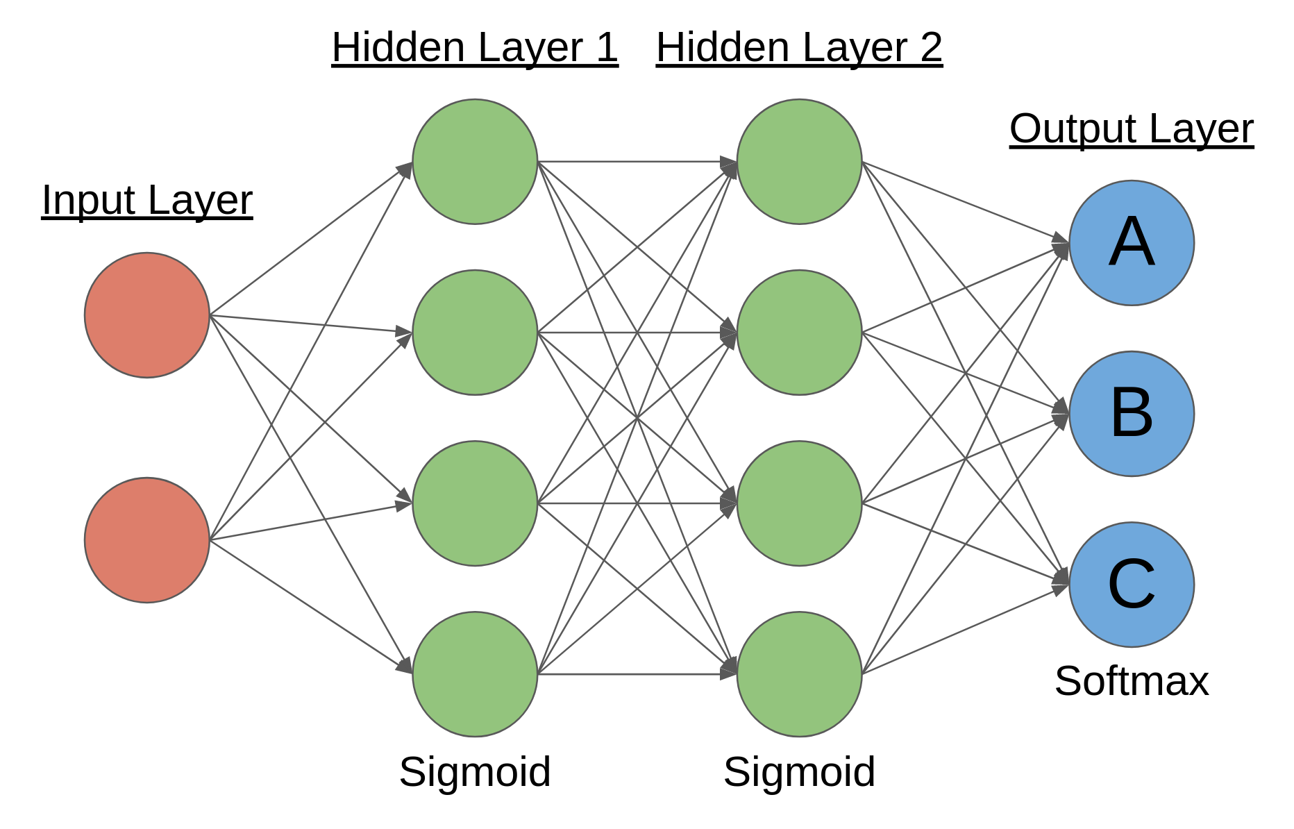
Deep neural network diagram for classification; uses 2 hidden layers
Each of those circles is called a neuron, and is the fundamental unit in a neural network. The leftmost layer is called the input layer, and its values are determined by the data inputs given. The rightmost layer is known as the output layer, and its values are the network’s prediction or strategy regarding the given inputs. In this case, the output neurons are each labeled with a different letter, symbolizing the different classes the input could be sorted into. This makes the network a classification network. Every layer in-between the input layer and the output layer is known as a hidden layer. If you recall from the definition, deep learning simply refers to neural networks which have 2 or more hidden layers, like in the diagram above.
The arrows between neurons represent connections. They connect the output of a neuron from a previous layer to a neuron in another layer as an input. Thus, in a simple feed-forward network like this, information passes from left to right as inputs are transformed into outputs. Each neuron performs a simple operation by itself, but through the powerful complexity provided by connections, the network can result in complex output overall.
So what does each neuron actually do? It actually only does two things; it takes a weighted sum of its inputs, then it passes the sum through a nonlinear activation function. The diagram below illustrates a simple case of this:
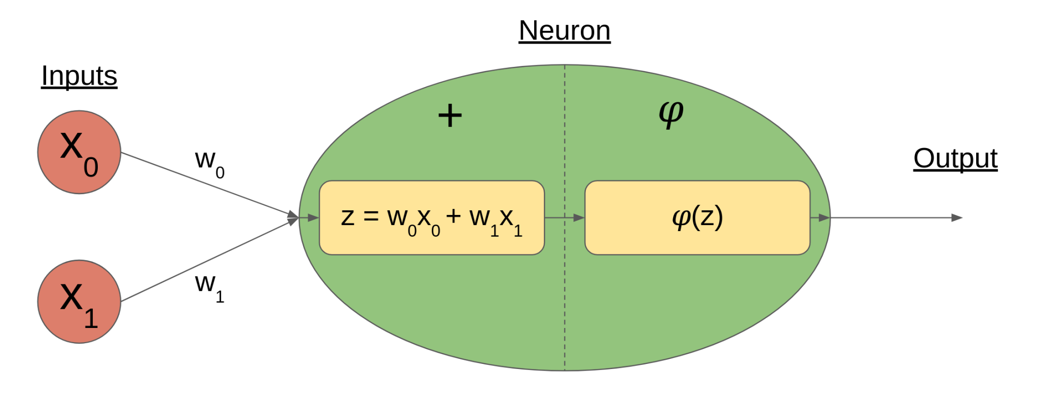
Neuron diagram showing weighted sum stage (+) and activation function stage (𝜑)
Here, the inputs to the neuron are the x variables, indexed from 0. Each input x has a corresponding weight w, such that the inputs’ summation z is more dependent on some inputs than others. This allows neurons to “learn” by identifying which features are most relevant to the problem it’s trying to solve. After the weighted sum is taken, it is passed through an activation function 𝜑 before the output is finalized.
When I first read about this process within each neuron, I was quite confused. The weighted sum part seemed simple enough, since its a logical way to combine small results from prior operations into a new result of larger scope. But why pass that through an activation function? Kelleher justifies it succinctly by saying this:
"Modeling these [complex] relationships accurately requires that a network be able to learn and represent complex nonlinear mappings. So, in order to enable a neural network to implement such nonlinear mappings, a nonlinear step (the activation function) must be included within the processing of the neurons in the network.”
Essentially, activation functions are the nonlinear spice which turn neural networks from dull linear models into robust nonlinear models. Without them, neural networks would just be a very fancy way to fit lines to data, a process which makes sense in very few scenarios. By adding nonlinearity into the mix, the networks can fit a much larger range of situations, which is where the point from the Data section about low bias comes from. Deep neural networks are thus a class of highly flexible, complex functions built out of deceptively simple components.
3. Measure of fitness
So now we know how neural networks turn inputs into outputs, but just how good are those outputs? In a real world scenario where the network must make predictions, the correct answer may not be known, and so this question becomes fairly futile. However, it is actually quite a simple problem during the network’s training stage, when the network is still “learning” relationships in the data. Here, we will assume that the network is performing supervised learning, where there is a desired output contained in the training data.
Let us define for a single input the desired output as a vector y of dimension N. Similarly, we define the network’s output vector ŷ, which is also of dimension N. Then, the error formula for the network is given by this simple formula:

SSE formula for network output ŷ and desired output y
See, it’s not so scary! All it’s doing is taking the difference between each element of the desired output and the network output, and then squaring it. Those squared differences are then summed up and multiplied by 1/2 to give the total error. That’s why it’s called the SSE formula; it stands for the Sum of Squared Errors. As an aside, the 1/2 factor makes no real difference to the error rankings, but it does make some of the math in the refinement mechanism a bit cleaner.
With this handy formula, network performance can be easily computed for one case, or averaged across multiple cases. Lower error rates mean that the network performed better overall, and thus demonstrates greater fitness to the problem at hand. This makes it easy to compare the performance of multiple networks attempting to solve the same problem, which is a crucial requirement for improving the network.
4. Refinement mechanism
Okay, things are all starting to come together now. We’ve covered what deep learning is for, what the models look like, and how to measure their fitness. And yet, we still have to answer a crucial question: how does one find a well fit network?
Unlike most models used in ordinary statistics, deep learning is not a deterministic process. Rather, it is a stochastic process. Essentially, this means that random chance plays a role in determining the model’s final form. The same cannot be said for a deterministic model, such as a linear regression, which can be calculated exactly from the input points.
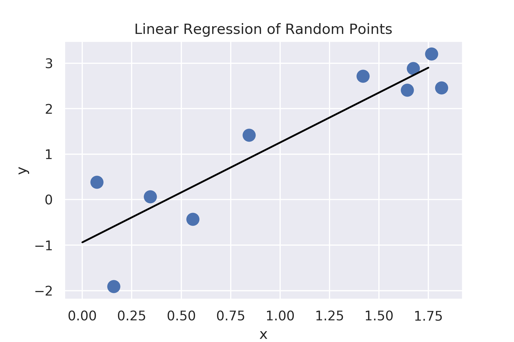
Unique result of linear regression on random points; x and y sampled from dependent normal distributions
The stochastic element of deep learning primarily stems from the initialization procedure, where random values are assigned to the network’s connection weights. This goes back to neural networks’ having distinctly low bias. Since these functions make very few assumptions before analyzing their data, it is only logical to reflect this through a random initialization. Of course, that random initial network probably does a terrible job at modelling the data. So how does it improve?
In short, it makes iterative improvements to each of its weights until performance cannot easily be improved. The two key algorithms behind this process are backpropogation and gradient descent. These related algorithms really deserve their own article to fully explore their mathematical origins. However, they can be described quite conveniently by analogy, as Kelleher does near the end of the book:
"An intuitive way of understanding [gradient descent] is to imagine a hiker who is caught on the side of a hill when a thick fog descends. Their car is parked at the bottom of the valley; however, due to the fog they can only see a few feet in any direction. Assuming that the valley has a nice convex shape to it, they can still find their way to their car, despite the fog, by repeatedly taking small steps that move down the hill following the local gradient at the position they are currently located.”
In this analogy, the hiker represents the network’s current state, and each position on the hill represents a different set of connection weights. His elevation above the valley floor represents his current error level, so going lower into the valley represents attaining better performance by modifying network connections. Though it is impossible to find the lowest point in the valley from a bird’s-eye view, he can know that he is getting lower by only taking steps which lead downhill. Then, by taking many steps, he can slowly work his way down into the valley even without seeing the path clearly from the start.
Neural networks refine their weights in a similar way. By using some clever mathematics, they can see how much each weight should be increased or decreased to reduce error slightly. General performance improves with each step, though not by much. It is only through repeatedly making these small adjustments that error is significantly lowered and a useful network finally results.

Foggy mountain gradient descent; note that it is impossible to find the lowest valley without walking down into them all
It should be noted that oftentimes there is more than one valley in this analogous scenario. Depending on which hillside the hiker starts on, he may end up in a different one, with no way of knowing if a lower one exists. Similarly, networks may find a configuration which cannot be improved by simply taking more small steps, though a better overall configuration exists. For this reason, multiple networks with different initialization configurations are often trained and their performances compared. This is a simple method to increase the probability that one of them hits the lowest valley’s floor.
Recap
This post has covered a lot of ground at once in attempting to describe deep learning, so it is probably best to give a brief review of everything that we’ve dealt with here. We started off by defining “artificial intelligence,” “machine learning,” and “deep learning,” showing how they are overlapping terms used to describe different algorithms aimed to mimic human reasoning. Deep learning refers to using a specific type of neural network to “learn” from data by matching feature relationships to a well fit function.
Next we discussed some of the goals of deep learning, whether it’s supervised, unsupervised, or reinforcement learning. This determines whether the user has a desired output at each step or in the long run.
Then we turned to each of the four “key ingredients” of deep learning individually. For reference, these are:
- Data
- Set of functions
- Measure of fitness
- Refinement mechanism
Through analyzing these components, we were able to break down some of the opaque processes that guide deep learning networks. They are highly flexible since they take advantage of large datasets, which are increasingly available due to the explosion of big data. In terms of structure, they are composed of many simple functions called neurons, which can generate complex, nonlinear behavior when they are combined. In order to find what connections lead to the best performance, an iterative refinement process is used, which is guided by a continual evaluation of the network’s error level. When all of these factors are combined, an incredibly adaptable function is created which can improve itself using data. In other words, it can learn.
These deep learning networks show great promise in many fields, even those which have long been thought to be beyond the scope of automation. Machines are certainly coming for both white collar and blue collar jobs, though in different forms. While robotic advances have already disrupted industrial labor, the real kicker that will be felt by a much broader segment of the workforce will stem from advances in machine learning. Teaching computers to think is no longer the stuff of sci-fi; it’s happening as we speak. Whether that results in a net gain or loss for society remains to be seen, but change is certain, and it is increasingly prudent to understand the processes facilitating that change. So keep thinking and learning as we all try to stay ahead of the machines, at least for a bit longer.
Data Science
Book Deep Learning Neural Networks