Sorting Stars
Learning about neural networks using stellar data
By Evan Meade, 2019-12-24

Stars are one of those things that seem simple from afar, but get ridiculously complex the closer you get. From Earth, just about every star looks like a perfect pinprick of light, uniformly white against a black background. Even the sun, a little bigger than the rest, looks like a nice round light bulb in the sky. Sadly, this simplistic view is far from reality.
Despite their similar appearances to the naked eye, stars vary wildly in terms of size, color, mass, temperature, brightness, and about a hundred other variables. Some are as massive as our sun, yet a million times smaller, emitting a brilliant white radiance. Others are ten times as massive, yet a billion times larger in volume. In short, there can be no singular description of what stars are like, since they vary widely in all relevant characteristics. How, then, can a model reflect this enormous variation without becoming impractically complex?
The trick, of course, is to simplify and classify.
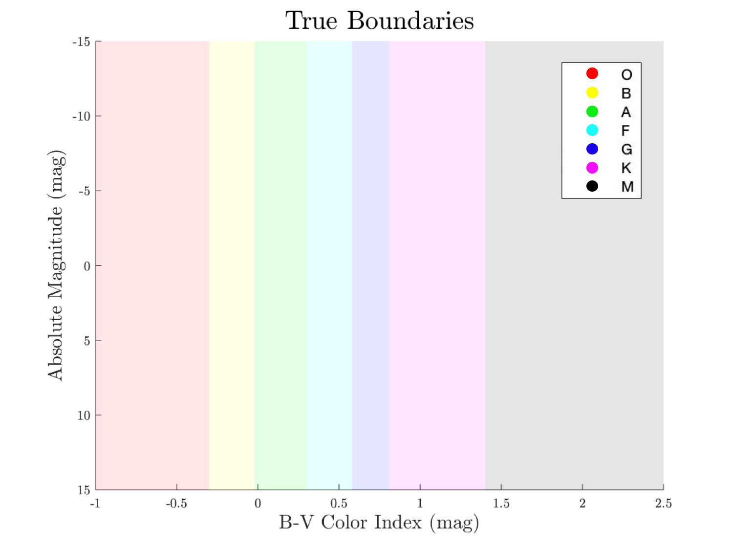
Hertzsprung-Russell diagram for spectral types O-M
The Hertzsprung-Russel diagram–also known as the HR diagram–is a handy tool to help cluster similar types of stars. The x-axis sorts by a stellar feature called the B-V color index, which is directly related to surface temperature. The y-axis corresponds to a star’s absolute magnitude, which is similar to brightness; more negative numbers correspond to greater brightness. Based on a star’s position in this feature space, it is classified as a certain “spectral type,” ranging from O to M for most common stars.
For a recent project, some colleagues and I had to use a scientific programming language called MATLAB to solve some problem. Our group consisted of Victoria Catlett (Physics and Math), Amanda Ehnis (Physics), and myself, Evan Meade (Physics and Math). Given our common interests in astrophysics and machine learning, we decided to create neural networks which could classify stars based on these features.
Motivation
We live in a Renaissance of Big Data, where we have exponential growth in the amount of recorded information year after year. However, without sufficient analysis to place this data in context, it remains relatively meaningless information. The sciences in particular have suffered from an explosion of raw data without a parallel expansion of data analysis. In short, we know a lot about what things are, but not what they mean. Nate Silver, a professional statistician and editor-in-chief of the political forecasting blog FiveThirtyEight describes this dilema perfectly:
“Meanwhile, if the quantity of information is increasing by 2.5 quintillion bytes per day, the amount of useful information almost certainly isn’t. Most of it is just noise, and the noise is increasing faster than the signal. There are so many hypotheses to test, so many data sets to mine-but a relatively constant amount of objective truth.”
With this project, my team and I hoped to improve our skills in data analysis, in order to better make use of the amazing developments in scientific research we will encounter both now and in the future. In particular, we wanted to use machine learning to classify spectral types because, although it is often misunderstood, it has great potential to allow for the efficient processing of massive datasets. This project specifically was a great way to build those skills in a controlled environment because it is a relatively simple problem which still has its own unique challenges.
Data
The first step in any successful machine learning project is to acquire a large, high-quality dataset. Luckily, astrophysics is a data-rich field, with most datasets being publicly available. In this case, we used the Hipparcos, Yale, and Gliese (HYG) catalog, which compiles a large number of features from multiple astronomical databases. The combination of these datasets is a huge catalog, with N = 115,015.
For our project, we chose to isolate 2 input features: B-V index and absolute magnitude. Because spectral type is directly related to position in this feature space, we believed that these were the most pertinent features to classifying stars correctly, and that using any more would result in overfitting to noisy patterns. We also extracted 1 target feature from the HYG dataset: spectral type. This was an obvious decision since it was the very feature we were trying to predict from the input features. When all of these features are plotted together, a beautiful plot emerges showing how these regions border and even overlap.
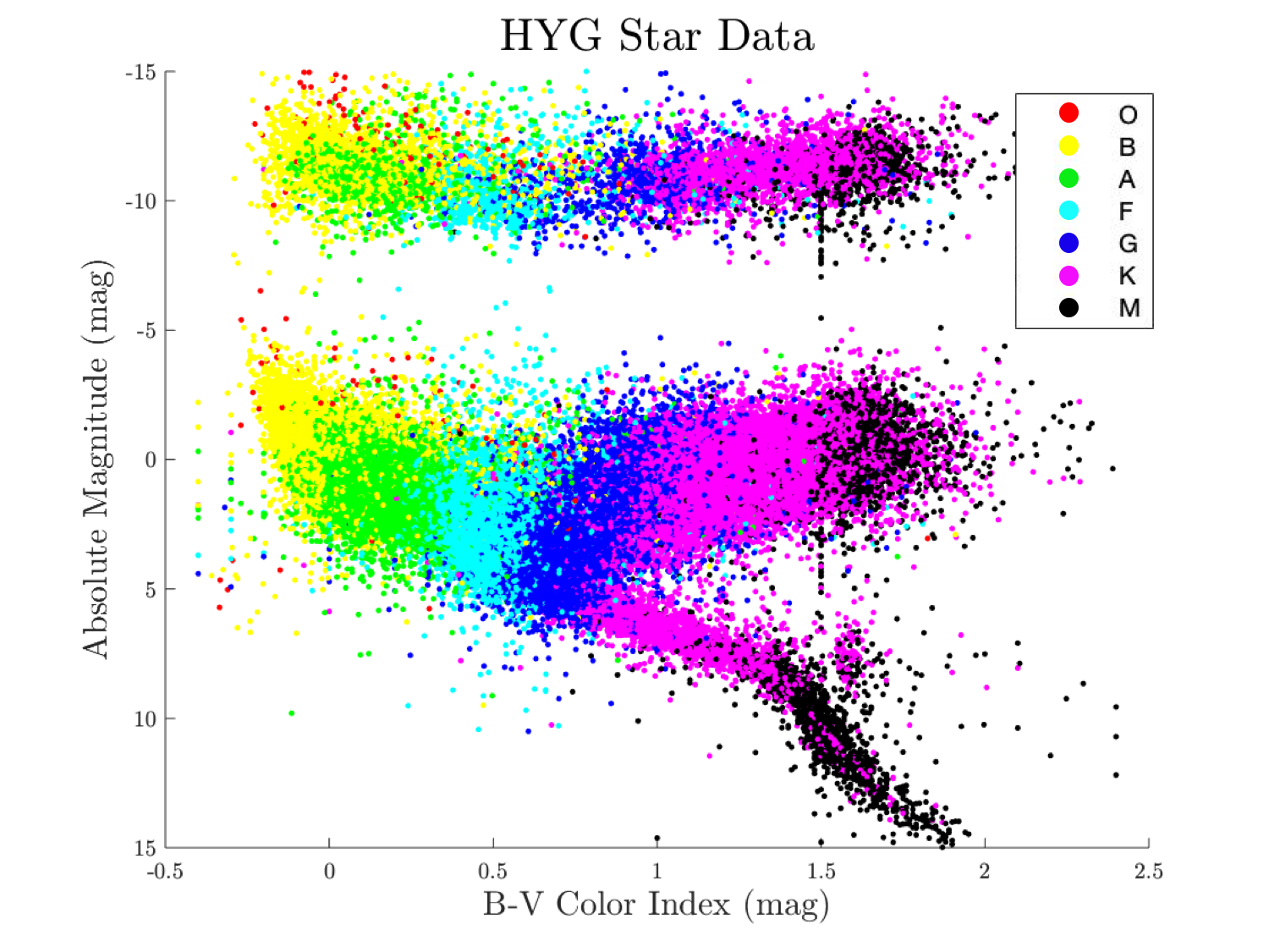
HYG data plotted on an HR diagram
It should be noted that due to a combination of measurement errors and physical variation, these spectral classifications do not perfectly align with the neat vertical classification regions in the earlier figure. However, they still largely fit the pattern of vertical columns determined by B-V index, so an effective neural network can still be constructed provided the prediction question can be posed quantitatively.
In order to translate spectral type into a form that a neural network can understand, we created a set of seven “dummy variables.” Dummy variables are a set of binary variables, each of which corresponds to a different class type, in this case one each for O, B, A, F, G, K, and M. For each star, its corresponding class is marked with a 1 and the rest are set to 0. This allows a categorical variable to be transformed into a set of quantitative variables, which can then be processed by a neural network.
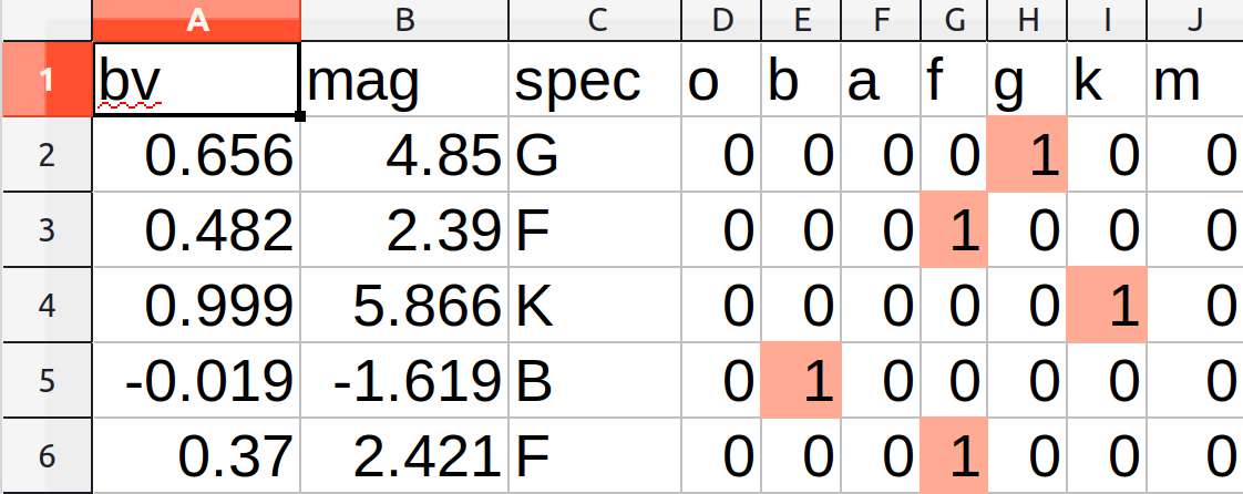
Dummy variables for spectral type in HYG data
Methods
Our team implemented a variety of neural networks to compare and contrast their performance and convenience. However, for the sake of clarity, this article will only focus on our use of built-in methods from the Deep Learning Toolbox™ in MATLAB. Our full report, along with our code and data, can be found on our project’s GitHub repository.
This Toolbox contains a lot of useful functions for quickly constructing and training neural networks, which are algorithms modeled loosely after the human brain.
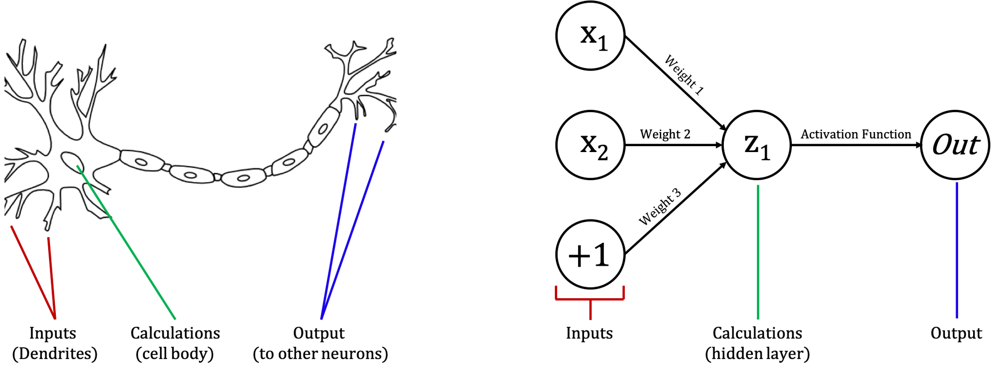
A neuron and its analogies to a simple neural network with inputs, calculations, and outputs; neuron image from Virtual Amrita Laboratories
At each neuron, input values are combined into a weighted sum, along with a weighted constant known as a “bias.” In this way, the sum represents a higher dimensional equivalent of a line, which can be written in a form such as y = mx + b. Thus, the “knowledge” of any given neural network is effectively stored in the weights between neurons, which represent how much one affects the other.
Once this weighted sum is calculated, it is passed through a nonlinear function called an activation function. This allows the network to model more complex situations where linear models don’t necessarily apply. In theory, any nonlinear function can be used to this effect, though in reality only a handful are commonly used. Examples of common activation functions include the sigmoid, hyperbolic tangent, and rectified linear functions.

Common activation functions: sigmoid, hyperbolic tangent, and rectified linear functions
By combining a number of simple functions–known as neurons–a complex model can emerge which correctly classifies or predicts data. The beauty of machine learning is that the training algorithm selects the necessary parameters automatically. There are only three things the human experimenter needs to provide in order to facilitate this automated learning. According to Dr. John D. Kelleher from the Technological University Dublin, these are:
“1. Data (a set of historical examples).
2. A set of functions that the algorithm will search through to find the best match with the data.
3. Some measure of fitness that can be used to evaluate how well each candidate function matches the data.”
The first point is easy enough in this case; we quickly found a large, high-quality dataset from the HYG catalog. The second point, however, opens the door to a lot more choice. The set of possible functions for a neural network is determined by its size and connections. In particular, how many layers it has, how many nodes are in each layer, and what activation functions are used between each layer.
By default, MATLAB’s Toolbox uses a “shallow” neural network for classification. This just means that there is only one layer of neurons between the input and output layers. Additionally, the activation functions are already set. The hidden layer uses the sigmoid activation function, which is pretty standard, but increasingly unpopular compared to other functions like the rectified linear function. Meanwhile, the output layer uses the softmax activation function, which exponentially weights and normalizes activations such that all output probabilities sum to 1. This is perfect for any kind of classification network, since it can help show how likely a case is to belong to any particular class. All put together, the network looks something like this:
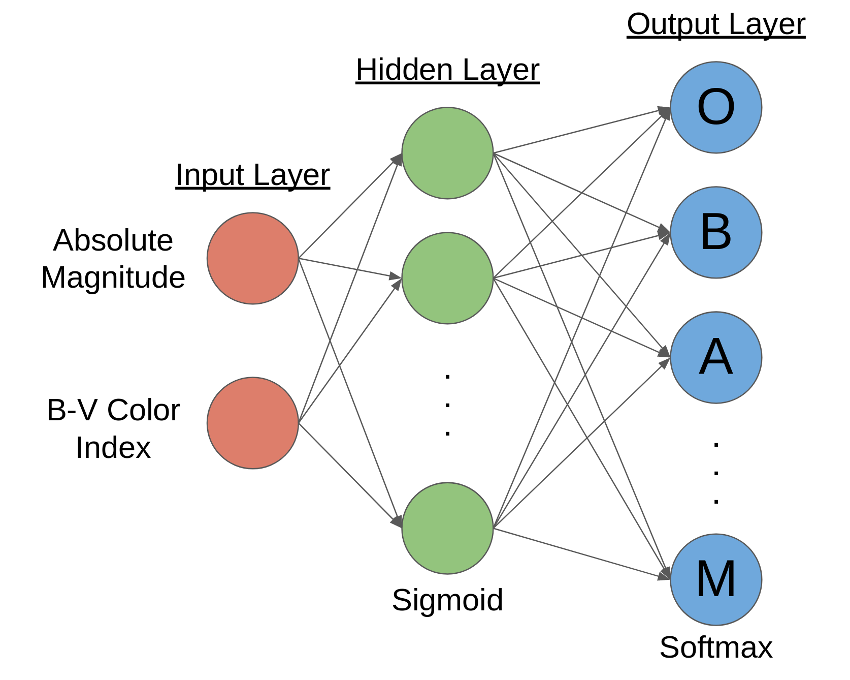
Neural network architecture for star classification using MATLAB’s Deep Learning Toolbox™
Returning briefly to the 3rd ingredient in successful machine learning, MATLAB defaults to using the “cross-entropy” evaluation function. This method assigns 0 error to correct predictions, while growing exponentially higher to infinity for incorrect predictions. Thus, it penalizes most those categories which are furthest from the target values of their dummy variables.
Finally, with all these components in place, the whole process is enabled with the particular learning algorithm, which in this case is the “scaled conjugate gradient” method. The math behind this process really deserves its own article, but at its most basic level, it is an efficient way of adjusting parameters to minimize error.
Performance
In order to see how different network configurations and training scenarios affected overall performance, I varied these parameters over a decent domain and averaged results over multiple runs of each configuration. Specifically, I varied the hidden layer size and the percentage of the HYG dataset that was used for training. Factors like these are sometimes referred to as hyperparameters, because they are manually set values which shape the range of possible networks.
I tried every hidden layer size from 1 to 24 neurons, and training percentages of 50, 60, 70, 80, and 90%. For each of these hyperparameter combinations, I averaged results over 10 runs. This is because the random initialization of neural networks means that performance of a particular network may be significantly influenced by chance. Statistical results, such as the central limit theorem, tell us that this variability can be reduced by averaging over multiple runs. In total, it took my i7 quad-core laptop about 10 hours to train and test all of these networks, giving some fascinating trends in the results.
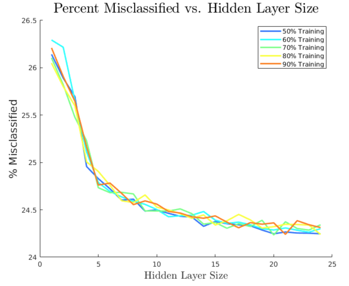
Percentage of test stars misclassified, averaged over 10 networks per configuration
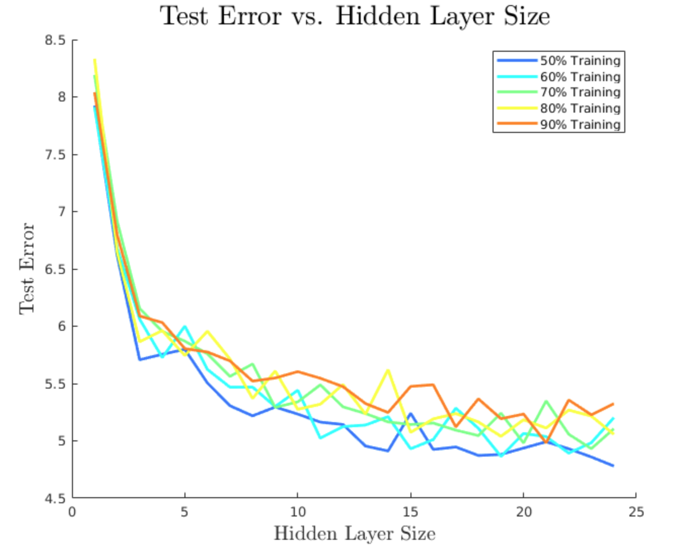
Cross-entropy error for test stars, averaged over 10 networks per configuration
Three key takeaways may be seen from these charts. First, we can clearly see that larger hidden layers decreased the error and misclassification rates on average, but also demonstrated declining returns to an asymptotic limit. This makes sense because larger hidden layers mean more connections weights, which are effectively what store the information of any particular model. Thus, larger networks can store smaller details about feature relationships, which refine the model’s accuracy. However, natural error and variance means that even an optimally trained network can never achieve perfect accuracy in modelling physical systems. Performance can only get so good, as indicated by the flattening out of all curves as size increases.
Second, we can see that lower training percentages actually resulted in better performance on average. This result is counterintuitive, because one would normally expect that more information would result in a more accurate model. However, the presence of noise or extraneous variables, as explained in the next few sections, can result in models which fit random trends in training data, decreasing overall performance in the testing stage.
Finally, for lack of a better word, we can see significant bumpiness in the curves even though they are averaged over 10 networks each. This demonstrates neural networks’ sensitivity to initial conditions. Randomness in initial parameters and train/test splits of the data creates inherent variability in network performance, which is reflected in the noise of these performance curves.
Things we did right
- We used a large, high-quality dataset – One of the trade-offs in machine learning is between fitting functions to data versus bias. Bias, in its most basic sense, is any preconceived notion about a data’s structure. For instance, a linear model is heavily biased because it assumes that one variable directly affects another at a constant rate. As a consequence, effective linear models can be fit with relatively small amounts of data. By contrast, neural networks assume very little about data since they can theoretically model any nonlinear relationship. Consequently, they require large amounts of reliable data to “learn” the variables’ relationships.
- We trained many networks with varied parameters – Despite how it is sometimes portrayed, machine learning models are not magic bullets. There is no guarantee that any particular neural network will have optimal performance. Adjusting different hyperparameters, such as training percentage and hidden layer size, can reveal what types of networks do best. However, chance always plays a role, since unlike a deterministic model like least squares, neural networks are stochastic due to the randomness of initial parameters and train/test splits. By testing average performance over this input space, we were able to find better performing networks than if we settled for the first network we trained.
Things we did wrong
- We probably overfit the model – Overfitting is a modelling flaw where a model is matched too heavily to training data, thereby decreasing overall accuracy in the testing phase. It often results from a model being overly complex to describe a simpler phenomenon. The key sign of overfitting here is that networks with lower training percentages generally did better than ones with higher training percentages. This is a paradoxical result where adding more information actually made our models worse, when a good model may be expected to get better or at least remain the same.
- We probably used too many inputs – Because spectral type is a human-defined feature, we had the advantage of knowing what exactly defined it. As shown in the “True Boundaries” diagram, it is essentially just dependent on a star’s B-V index. For that reason, we likely over-complicated the model by including absolute magnitude as an input feature when it has no physical relationship to spectral type. As a result, the network likely fit noise in the absolute magnitude data, resulting in the overfitting phenomenon described above.
Conclusions
Machine learning, particularly with neural networks, is clearly a very powerful tool for deriving real insights even from noisy data. Its greatest advantage is its ability to derive meaningful features from large datasets with minimal direction from the user. A few simple “hyperparameters,” which determine the neural network’s structure, describe the kinds of functions which can be fit. By combining this architecture with a large amount of data and an evaluation metric, networks can be optimally trained using algorithms which reduce overall error.
In this particular project, my team and I showed how shallow neural networks–those consisting of only one hidden layer between inputs and outputs–can effectively classify stars by spectral type. In the process of experimenting with networks, we learned a lot about how they can be used to help process observational data.
To anyone considering using neural networks in an upcoming project, I would advise you to carefully consider whatever data you feed the network. To state the obvious, neural networks model whatever relationships exist in the training set, and as a result, they are highly susceptible to modelling noise. It is therefore up to the human user to help distinguish meaningful from meaningless inputs in each particular case. When it comes to machine learning, you always reap the model of the data you sow.
Data Science
Astrophysics MATLAB Stars